ABSTRACT
Categorical outcome analyses in randomized controlled trials (RCTs) and observational studies are commonly presented as relative risks (RRs) and odds ratios (ORs). In some situations, these RRs and ORs may be misunderstood, resulting in wrong conclusions. How this may happen is explained in the context of a hypothetical RCT that compares potentially lifesaving drugs A and B with placebo. In this RCT, the RR for survival is 1.67 for A vs placebo and 1.42 for B vs placebo. Using these RR data, as a challenge, readers are invited to answer 2 questions either intuitively or by other means. First, by how much is A better than B? Second, if the absolute survival rate with B is 8.5%, using the answer obtained from the previous question, what is the absolute survival rate with A? In this same RCT, the OR for survival is 1.74 for A vs placebo and 1.46 for B vs placebo. Using the OR data instead of the RR data, readers are again invited to answer the 2 questions listed above. This article explains why it is easy for readers and even authors to arrive at wrong answers to the 2 questions and draw wrong conclusions about the results. This article also explains what the correct answers are and how they may be obtained. The explanations involve simple concepts and even simpler arithmetic.
J Clin Psychiatry 2023;84(3):23f14943
Author affiliations are listed at the end of this article.
The absolute risk of an event is the probability that it will occur. The relative risk (RR) of an event is the probability that it will occur in the group of interest relative to (ie, divided by) the probability that it will occur in a reference (comparison, control) group. Statistics such as the RR, odds ratio (OR), and hazard ratio (HR), along with their 95% confidence intervals (CIs), were explained in earlier articles in this column and elsewhere.1–4 These statistics are very easy to understand, and readers who are unfamiliar with their meaning and derivation may wish to refer to these previous articles before continuing with the present one.
The present article is also very easy to understand and involves only simple operations such as subtraction and division. The article is long only because the explanations are simplified and therefore detailed. Readers are encouraged to keep pen and paper by their side and to work out for themselves what is explained; this will consolidate the understanding of concepts.
To answer the questions posed to readers in the Abstract of this article, using the RRs provided, it can be deduced that A is 18% better relative to B and that if the absolute survival rate is 8.5% with B, absolute survival with A will be 1.5% higher, making the absolute survival rate 10% with A. Importantly, the questions posed cannot be answered using the ORs. The rest of this article presents the explanations.
Understanding the Results
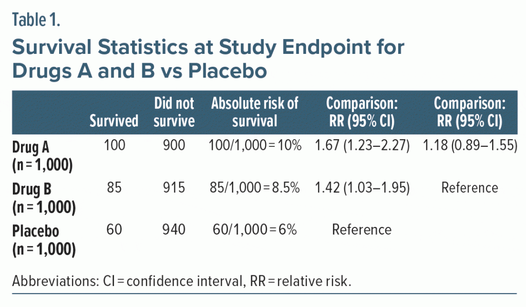
Consider a hypothetical large (n = 3,000) randomized controlled trial (RCT) that tests two experimental drugs, A and B, against placebo for a disease that has a very high fatality rate. At the 6-month study endpoint, both A (RR, 1.67; 95% confidence interval [CI], 1.23–2.27) and B (RR, 1.42; 95% CI, 1.03–1.95) resulted in superior survival rates relative to placebo (Table 1).
As a digression for student readers, in Table 1, columns 2 and 3 present the raw data. Column 4 tells us the absolute risk of survival and how it was calculated. The RRs in column 5 can be calculated using pen and paper or an ordinary calculator: 10%/6% gives us 1.67 and 8.5%/6.0% gives us 1.42. The 95% CI can be obtained using any free online calculator for the RR; this is quicker and easier than manual calculation.
Continuing the digression, we don’t need to look at P values to understand that survival with drugs A and B was significantly superior to that with placebo. First, we recognize that if there is “no difference” in survival between A and placebo (ie, survival rates are identical), the RR will be 1.00. This is because if division is performed with identical numbers, the result is 1.00. Next, we observe that the RR for survival with A is 1.67. This is higher than 1.00, the value for “no difference.” So, A is associated with a higher “risk” (probability) of survival. Finally, the entire 95% CI for this RR, 1.23–2.27, lies above 1.00. This indicates that we are reasonably sure that the population value for the RR is above 1.00, and this leads us to conclude that A is significantly superior to placebo (P < .05). We draw similar conclusions from the RR and its 95% CI for drug B. In summary, we can understand whether an RR is statistically significant or not by looking at where its 95% CI lies with regard to 1.00, the value for “no difference.”
Returning to Table 1, we draw 2 correct conclusions from the results presented in column 5. One is that, with regard to survival, A is 67% better than placebo. The other is that B is 42% better than placebo. These conclusions can be arrived at in 2 ways. The shorter way is to observe that 1.67–1.00 is 0.67 or 67% and that 1.42–1.00 is 0.42 or 42%.
As a digression for student readers, why do we subtract 1.00? When we earlier calculated the RR to be 10%/6% and obtained 1.67, the reference (placebo) group denominator was standardized to a value of 1.00. Just as a value of 10/6 means that the numerator exceeds the denominator by 4 (relative to 6), a value of 1.67 means that the numerator exceeds the denominator by 0.67 (relative to 1.00).
The longer way to draw the same conclusion is to observe from Table 1, column 4, that survival was 10% with A and 6% with placebo (reference). That is, survival was 4% better with A. With a few seconds of mental arithmetic, we determine that 4% is 0.67 or 67% of the reference value (6%).
Misunderstanding the Results
To recapitulate, from column 5 in Table 1, we correctly concluded that A improved survival by 67% relative to placebo and that B improved survival by 42% relative to placebo. Because both these values were obtained by subtracting the same quantity (the value for placebo), it may seem intuitively correct to subtract B from A (42 from 67) and conclude that A is 25% better than B as the answer to the first question posed in the Abstract.
The automatic assumption when we draw such a conclusion is that A is 25% better than B with reference to B. Under this assumption, such a conclusion is completely wrong because the 25% value was obtained with placebo in the denominator whereas the “with reference to B” assumes that B is the denominator (this is explained further in the next section). The conclusion is correct only under the assumption that A is 25% better than B with reference to placebo because the RRs 1.67 and 1.42 were both calculated with reference to placebo.
How do we understand this? In Table 1, column 4, we see that A is better than B by 1.5%, and 1.5 is a quarter (25%) of 6%, the value for placebo in column 4.
Another way of understanding this is to consider that RRs of 1.67 and 1.42 mean that, if survival with placebo is 1.00, survival with A is 1.67 with reference to 1.00 and survival with B is 1.42 with reference to 1.00. So, survival in A is better than survival in B by 0.25 with reference to 1.00; that is, placebo. Because this is not necessarily intuitive, a frequent mistaken interpretation is that A is better than B by 0.25 with reference to B.
Another intuitive and again wrong approach is to directly compare improvement with A and that with B and conclude that A is 59% better than B because 67/42 gives 1.59. This approach is wrong because, as explained in the next section, we should be dividing 1.67 by 1.42 and not 67 by 42. Note that there is no alternate interpretation that would yield 59% as a result.
Correcting the Misunderstandings
How did we obtain the RR values that are presented in column 5? We divided absolute risks (column 4) for drug vs placebo, as explained in an earlier section. Likewise, if we want to compare the chances of survival between A and B we must divide the absolute risks (column 4) for A and B. When we divide 10.0 by 8.5, we obtain 1.18, which is what we see in column 6. Note that when we divide (not subtract) 1.67 by 1.42 (column 5) we get this same value: 1.18. So, survival with A is 18% better than survival with B (relative to B). To answer the second question posed in the Abstract, if absolute survival with B is 8.5%, 18% of 8.5% gives us 1.5%. So, absolute survival with A is (8.5% + 1.5%) or 10%.
As a digression for student readers, A may be 18% better than B, but it is not better to a statistically significant extent. We can understand this when we look at the 95% CI, 0.89–1.55, in column 6. This CI surrounds 1.00, the value for “no difference.” The CI tells us that it is likely that the population value for the RR lies below 1 by as much as 11%, is equal to 1, or exceeds 1 by as much as 55%. That is, A may be associated with poorer survival, equal survival, or better survival than B. Obviously, A cannot be “significantly” better than B if it is also possible that it is no different from or worse than B.
Note that survival with A is 18% better than survival with B in relative terms. In absolute terms, from column 4 we see that survival with A was better by only 10.0–8.5; that is, 1.5%. We can convert this value of 1.5% into a relative value: A was better than B by 1.5%, B was associated with 8.5% survival, so A was better than B by 1.5/8.5 or 18%. The answer is the same as that obtained by other means, described above.
In summary, the wrong conclusions are that A is 25% or 59% better than B with reference to B. The right conclusions are that A is 1.5% better than B in absolute terms and 18% better than B in relative terms.
Understanding Why the Misunderstanding Occurs
In studies such as this, and in cohort and case-control studies in which data of a similar nature are presented in journal papers, most or all of the relevant data are presented in tables, as presented for our hypothetical study in Table 1. However, what is highlighted in the abstract of the papers, and in the discussion of the results, is only the information that is shown in column 5. Information such as that shown in column 4 is sometimes but not always presented, and information that is presented in column 6, the subject of the present article, is almost never presented. So, readers use their intuition and draw their own conclusions, and, as this article points out, intuition and conclusions can sometimes be wrong.
Authors May Also Draw the Wrong Conclusions
It is not readers, alone, who may misinterpret findings; sometimes, authors also do so, even in studies published in leading journals. As an example, in a nested case-control study of breast cancer in women with schizophrenia, Taipale et al5 subtracted the risk associated with prolactin-sparing antipsychotics (OR = 1.19) from the risk associated with prolactin-raising antipsychotics (OR = 1.56) and concluded that the use of prolactin-raising antipsychotics was associated with a 37% relative increase in the odds of breast cancer. They then used this number (37%) to estimate the probable impact of prolactin-increasing antipsychotics on the risk of breast cancer in the general population. Their conclusions, based on incorrect calculations, were far-reaching but incorrect.
End Notes
Some of what has been presented in this article with regard to the RR also applies to statistics such as the OR and HR. For example, with reference to the numbers in columns 2 and 3 in Table 1, the ORs are 1.74 (95% CI, 1.25–2.42) for A vs placebo and 1.46 (95% CI, 1.03–2.05) for B vs placebo. When A is compared with B, the OR is 1.20 (0.88–1.62), and this same value can be obtained by dividing A by B (1.74/1.46 = 1.19); the small difference is due to rounding error.
Some of what has been presented in this article with regard to the RR does not apply to statistics such as the OR; for example, subtracting the OR for B from that for A, we get 0.28, which does not represent anything that we have seen in this article. This is because ORs cannot be added or subtracted.
Why can’t we subtract ORs? Here is the explanation for those who might be interested. In Table 1, the OR for A vs placebo is (100:900)/(60:940); this converts to (100 × 940)/(900 × 60), or 1.74. Note that the denominator is (900 × 60). The OR for B vs placebo is (85:915)/60:940); this converts to (85 × 940)/(915 × 60), or 1.46. Note that the denominator is (915 × 60); this is different from the denominator for A vs placebo. With ratios, when the denominators are the same, denominators can be ignored when the ratios (or their numerators) are added or subtracted. We saw that this is true for the RR. When denominators are different, as for ORs, they cannot be ignored; they need to be included in the mathematical operations.
Article Information
Published Online: June 5, 2023. https://doi.org/10.4088/JCP.23f14943
© 2023 Physicians Postgraduate Press, Inc.
To Cite: Andrade C. Understanding misunderstandings about the relative risk and odds ratio. J Clin Psychiatry. 2023;84(3):23f14943.
Author Affiliations: Department of Clinical Psychopharmacology and Neurotoxicology, National Institute of Mental Health and Neurosciences, Bangalore, India ([email protected]).
 Each month in his online column, Dr Andrade considers theoretical and practical ideas in clinical psychopharmacology with a view to update the knowledge and skills of medical practitioners who treat patients with psychiatric conditions.
References (5)

- Andrade C. Understanding relative risk, odds ratio, and related terms: as simple as it can get. J Clin Psychiatry. 2015;76(7):e857–e861. PubMed CrossRef
- Andrade C. How to understand the 95% confidence interval around the relative risk, odds ratio, and hazard ratio: as simple as it gets. J Clin Psychiatry. 2023;84(3):23f14933.
- Andrade C. A primer on confidence intervals in psychopharmacology. J Clin Psychiatry. 2015;76(2):e228–e231. PubMed CrossRef
- Streiner DL. Risky business: making sense of estimates of risk. Can J Psychiatry. 1998;43(4):411–415. PubMed CrossRef
- Taipale H, Solmi M, Lähteenvuo M, et al. Antipsychotic use and risk of breast cancer in women with schizophrenia: a nationwide nested case-control study in Finland. Lancet Psychiatry. 2021;8(10):883–891. PubMed CrossRef
This PDF is free for all visitors!


